Flowsheet Continuous Stirred Tank Reactor (CSTR) Simulation and Optimization of Ethylene Glycol Production

Flowsheet Continuous Stirred Tank Reactor (CSTR) Simulation and Optimization of Ethylene Glycol Production#

Author: Brandon Paul
Maintainer: Brandon Paul
Updated: 2023-06-01

Learning Outcomes#

Call and implement the IDAES CSTR unit model
Construct a steady-state flowsheet using the IDAES unit model library
Connecting unit models in a flowsheet using Arcs
Fomulate and solve an optimization problem
- Defining an objective function
- Setting variable bounds
- Adding additional constraints

Problem Statement#

This example is adapted from Fogler, H.S., Elements of Chemical Reaction Engineering 5th ed., 2016, Prentice Hall, p. 157-160.

Ethylene glycol (EG) is a high-demand chemical, with billions of pounds produced every year for applications such as vehicle anti-freeze. EG may be readily obtained from the hydrolysis of ethylene oxide in the presence of a catalytic intermediate. In this example, an aqueous solution of ethylene oxide hydrolizes after mixing with an aqueous solution of sulfuric acid catalyst:

C₂H₄O + H₂O + H₂SO₄ → C₂H₆O₂ + H₂SO₄

This reaction often occurs by two mechanisms, as the catalyst may bind to either reactant before the final hydrolysis step; we will simplify the reaction to a single step for this example.

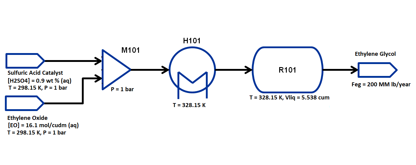
The flowsheet that we will be using for this module is shown below with the stream conditions. We will be processing ethylene oxide and catalyst solutions of fixed concentrations to produce 200 MM lb/year of EG. As shown in the flowsheet, the process consists of a mixer M101 for the two inlet streams, a heater H101 to preheat the feed to the reaction temperature, and a CSTR unit R101 with an external cooling system to remove heat generated by the exothermic reaction. We will assume ideal solutions and thermodynamics for this flowsheet, as well as well-mixed liquid behavior (no vapor phase) in the reactor. The properties required for this module are available in the same directory:

egprod_ideal.py
egprod_reaction.py

The state variables chosen for the property package are molar flows of each component by phase in each stream, temperature of each stream and pressure of each stream. The components considered are: ethylene oxide, water, sulfuric acid and ethylene glycol and the process occurs in liquid phase only. Therefore, every stream has 4 flow variables, 1 temperature and 1 pressure variable.

Importing Required Pyomo and IDAES components#

To construct a flowsheet, we will need several components from the Pyomo and IDAES packages. Let us first import the following components from Pyomo:

Constraint (to write constraints)
Var (to declare variables)
ConcreteModel (to create the concrete model object)
Expression (to evaluate values as a function of variables defined in the model)
Objective (to define an objective function for optimization)
TransformationFactory (to apply certain transformations)
Arc (to connect two unit models)

For further details on these components, please refer to the pyomo documentation: https://pyomo.readthedocs.io/en/stable/

From idaes, we will be needing the FlowsheetBlock and the following unit models:

Mixer
Heater
CSTR

We will also be needing some utility tools to put together the flowsheet and calculate the degrees of freedom, tools for model expressions and calling variable values, and built-in functions to define property packages, add unit containers to objects and define our initialization scheme.

from pyomo.environ import (
    Constraint,
    Var,
    ConcreteModel,
    Expression,
    Objective,
    TransformationFactory,
    value,
    units as pyunits,
)
from pyomo.network import Arc

from idaes.core import FlowsheetBlock
from idaes.models.properties.modular_properties import (
    GenericParameterBlock,
    GenericReactionParameterBlock,
)
from idaes.models.unit_models import Feed, Mixer, Heater, CSTR, Product

from idaes.core.solvers import get_solver
from idaes.core.util.model_statistics import degrees_of_freedom
from idaes.core.util.initialization import propagate_state

Importing Required Thermophysical and Reaction Packages#

The final step is to import the thermophysical and reaction packages. We have created a custom thermophysical package that support ideal vapor and liquid behavior for this system, and in this case we will restrict it to ideal liquid behavior only.

The reaction package here assumes Arrhenius kinetic behavior for the CSTR, for which $k_0$ and $E_a$ are known a priori (if unknown, they may be obtained using one of the parameter estimation tools within IDAES).

$ r = -kVC_{EO} $, $ k = k_0 e^{(-E_a/RT)}$, with the variables as follows:

$r$ - reaction rate extent in moles of ethylene oxide consumed per second; note that the traditional reaction rate would be given by $rate = r/V$ in moles per $m^3$ per second
$k$ - reaction rate constant per second
$V$ - volume of CSTR in $m^3$, note that this is liquid volume and not the total volume of the reactor itself
$C_{EO}$ - bulk concentration of ethylene oxide in moles per $m^3$ (the limiting reagent, since we assume excess catalyst and water)
$k_0$ - pre-exponential Arrhenius factor per second
$E_a$ - reaction activation energy in kJ per mole of ethylene oxide consumed
$R$ - gas constant in J/mol-K
$T$ - reactor temperature in K

These calculations are contained within the property, reaction and unit model packages, and do not need to be entered into the flowsheet. More information on property estimation may be found in the IDAES documentation on Parameter Estimation.

ParamEst parameter estimation:

Let us import the following modules from the same directory as this Jupyter notebook:

egprod_ideal as thermo_props
egprod_reaction as reaction_props

import egprod_ideal as thermo_props
import egprod_reaction as reaction_props

Constructing the Flowsheet#

We have now imported all the components, unit models, and property modules we need to construct a flowsheet. Let us create a ConcreteModel and add the flowsheet block.

m = ConcreteModel()
m.fs = FlowsheetBlock(dynamic=False)

We now need to add the property packages to the flowsheet. Unlike the basic Flash unit model example, where we only had a thermophysical property package, for this flowsheet we will also need to add a reaction property package. We will use the Modular Property Framework and Modular Reaction Framework. The get_prop method for the natural gas property module automatically returns the correct dictionary using a component list argument. The GenericParameterBlock and GenericReactionParameterBlock methods build states blocks from passed parameter data; the reaction block unpacks using **reaction_props.config_dict to allow for optional or empty keyword arguments:

m.fs.thermo_params = GenericParameterBlock(**thermo_props.config_dict)
m.fs.reaction_params = GenericReactionParameterBlock(
    property_package=m.fs.thermo_params, **reaction_props.config_dict
)

Adding Unit Models#

Let us start adding the unit models we have imported to the flowsheet. Here, we are adding a Mixer, a Heater and a CSTR. Note that all unit models need to be given a property package argument. In addition to that, there are several arguments depending on the unit model, please refer to the documentation for more details on IDAES Unit Models. For example, the Mixer is given a list consisting of names to the two inlets.

m.fs.OXIDE = Feed(property_package=m.fs.thermo_params)
m.fs.ACID = Feed(property_package=m.fs.thermo_params)
m.fs.PROD = Product(property_package=m.fs.thermo_params)
m.fs.M101 = Mixer(
    property_package=m.fs.thermo_params, inlet_list=["reagent_feed", "catalyst_feed"]
)
m.fs.H101 = Heater(
    property_package=m.fs.thermo_params,
    has_pressure_change=False,
    has_phase_equilibrium=False,
)

m.fs.R101 = CSTR(
    property_package=m.fs.thermo_params,
    reaction_package=m.fs.reaction_params,
    has_heat_of_reaction=True,
    has_heat_transfer=True,
    has_pressure_change=False,
)

Connecting Unit Models Using Arcs#

We have now added all the unit models we need to the flowsheet. However, we have not yet specified how the units are to be connected. To do this, we will be using the Arc which is a pyomo component that takes in two arguments: source and destination. Let us connect the outlet of the Mixer to the inlet of the Heater, and the outlet of the Heater to the inlet of the CSTR. Additionally, we will connect the Feed and Product blocks to the flowsheet:

m.fs.s01 = Arc(source=m.fs.OXIDE.outlet, destination=m.fs.M101.reagent_feed)
m.fs.s02 = Arc(source=m.fs.ACID.outlet, destination=m.fs.M101.catalyst_feed)
m.fs.s03 = Arc(source=m.fs.M101.outlet, destination=m.fs.H101.inlet)
m.fs.s04 = Arc(source=m.fs.H101.outlet, destination=m.fs.R101.inlet)
m.fs.s05 = Arc(source=m.fs.R101.outlet, destination=m.fs.PROD.inlet)

We have now connected the unit model block using the arcs. However, we also need to link the state variables on connected ports. Pyomo provides a convenient method TransformationFactory to write these equality constraints for us between two ports:

TransformationFactory("network.expand_arcs").apply_to(m)

Adding Expressions to Compute Operating Costs#

In this section, we will add a few Expressions that allows us to evaluate the performance. Expressions provide a convenient way of calculating certain values that are a function of the variables defined in the model. For more details on Expressions, please refer to the Pyomo Expression documentation.

For this flowsheet, we are interested in computing ethylene glycol production in millions of pounds per year, as well as the total costs due to cooling and heating utilities.

Let us first add an Expression to convert the product flow from mol/s to MM lb/year of ethylene glycol. We see that the molecular weight exists in the thermophysical property package, so we may use that value for our calculations.

m.fs.eg_prod = Expression(
    expr=pyunits.convert(
        m.fs.PROD.inlet.flow_mol_phase_comp[0, "Liq", "ethylene_glycol"]
        * m.fs.thermo_params.ethylene_glycol.mw,  # MW defined in properties as kg/mol
        to_units=pyunits.Mlb / pyunits.yr,
    )
)  # converting kg/s to MM lb/year

Now, let us add expressions to compute the reactor cooling cost (\$/s) assuming a cost of 2.12E-5 \\$/kW, and the heating utility cost (\$/s) assuming 2.2E-4 \\$/kW. Note that the heat duty is in units of watt (J/s). The total operating cost will be the sum of the two, expressed in \$/year assuming 8000 operating hours per year (~10% downtime, which is fairly common for small scale chemical plants):

m.fs.cooling_cost = Expression(
    expr=2.12e-8 * (-m.fs.R101.heat_duty[0])
)  # the reaction is exothermic, so R101 duty is negative
m.fs.heating_cost = Expression(
    expr=2.2e-7 * m.fs.H101.heat_duty[0]
)  # the stream must be heated to T_rxn, so H101 duty is positive
m.fs.operating_cost = Expression(
    expr=(3600 * 8000 * (m.fs.heating_cost + m.fs.cooling_cost))
)

Fixing Feed Conditions#

Let us first check how many degrees of freedom exist for this flowsheet using the degrees_of_freedom tool we imported earlier. We expect each stream to have 6 degrees of freedom, the mixer to have 0 (after both streams are accounted for), the heater to have 1 (just the duty, since the inlet is also the outlet of M101), and the reactor to have 1 (duty or conversion, since the inlet is also the outlet of H101). In this case, the reactor has an extra degree of freedom (reactor conversion or reactor volume) since we have not yet defined the CSTR performance equation. Therefore, we have 15 degrees of freedom to specify: temperature, pressure and flow of all four components on both streams; outlet heater temperature; reactor conversion and volume.

print(degrees_of_freedom(m))

We will now be fixing the feed stream to the conditions shown in the flowsheet above. As mentioned in other tutorials, the IDAES framework expects a time index value for every referenced internal stream or unit variable, even in steady-state systems with a single time point $ t = 0 $ (t = [0] is the default when creating a FlowsheetBlock without passing a time_set argument). The non-present components in each stream are assigned a very small non-zero value to help with convergence and initializing. Based on stoichiometric ratios for the reaction, 80% conversion and 200 MM lb/year (46.4 mol/s) of ethylene glycol, we will initialize our simulation with the following calculated values:

m.fs.OXIDE.outlet.flow_mol_phase_comp[0, "Liq", "ethylene_oxide"].fix(
    58.0 * pyunits.mol / pyunits.s
)
m.fs.OXIDE.outlet.flow_mol_phase_comp[0, "Liq", "water"].fix(
    39.6 * pyunits.mol / pyunits.s
)  # calculated from 16.1 mol EO / cudm in stream
m.fs.OXIDE.outlet.flow_mol_phase_comp[0, "Liq", "sulfuric_acid"].fix(
    1e-5 * pyunits.mol / pyunits.s
)
m.fs.OXIDE.outlet.flow_mol_phase_comp[0, "Liq", "ethylene_glycol"].fix(
    1e-5 * pyunits.mol / pyunits.s
)
m.fs.OXIDE.outlet.temperature.fix(298.15 * pyunits.K)
m.fs.OXIDE.outlet.pressure.fix(1e5 * pyunits.Pa)

m.fs.ACID.outlet.flow_mol_phase_comp[0, "Liq", "ethylene_oxide"].fix(
    1e-5 * pyunits.mol / pyunits.s
)
m.fs.ACID.outlet.flow_mol_phase_comp[0, "Liq", "water"].fix(
    200 * pyunits.mol / pyunits.s
)
m.fs.ACID.outlet.flow_mol_phase_comp[0, "Liq", "sulfuric_acid"].fix(
    0.334 * pyunits.mol / pyunits.s
)  # calculated from 0.9 wt% SA in stream
m.fs.ACID.outlet.flow_mol_phase_comp[0, "Liq", "ethylene_glycol"].fix(
    1e-5 * pyunits.mol / pyunits.s
)
m.fs.ACID.outlet.temperature.fix(298.15 * pyunits.K)
m.fs.ACID.outlet.pressure.fix(1e5 * pyunits.Pa)

Fixing Unit Model Specifications#

Now that we have fixed our inlet feed conditions, we will now be fixing the operating conditions for the unit models in the flowsheet. Let us fix the outlet temperature of H101 to 328.15 K.

m.fs.H101.outlet.temperature.fix(328.15 * pyunits.K)

We’ll add constraints defining the reactor volume and conversion in relation to the stream properties. Particularly, we want to use our CSTR performance relation:

$V = \frac{v_0 X} {k(1-X)}$, where the CSTR reaction volume $V$ will be specified, the inlet volumetric flow $v_0$ is determined by stream properties, $k$ is calculated by the reaction package, and $X$ will be calculated. Reactor volume is commonly selected as a specification in simulation problems, and choosing conversion is often to perform reactor design.

For the CSTR, we have to define the conversion in terms of ethylene oxide as well as the CSTR reaction volume. This requires us to create new variables and constraints relating reactor properties to stream properties. Note that the CSTR reaction volume variable (m.fs.R101.volume) does not need to be defined here since it is internally defined by the CSTR model. Additionally, the heat duty is not fixed, since the heat of reaction depends on the reactor conversion (through the extent of reaction and heat of reaction). We’ll estimate 80% conversion for our initial flowsheet:

m.fs.R101.conversion = Var(
    initialize=0.80, bounds=(0, 1), units=pyunits.dimensionless
)  # fraction

m.fs.R101.conv_constraint = Constraint(
    expr=m.fs.R101.conversion
    * m.fs.R101.inlet.flow_mol_phase_comp[0, "Liq", "ethylene_oxide"]
    == (
        m.fs.R101.inlet.flow_mol_phase_comp[0, "Liq", "ethylene_oxide"]
        - m.fs.R101.outlet.flow_mol_phase_comp[0, "Liq", "ethylene_oxide"]
    )
)

m.fs.R101.conversion.fix(0.80)

m.fs.R101.volume.fix(5.538 * pyunits.m**3)

For initialization, we solve a square problem (degrees of freedom = 0). Let’s check the degrees of freedom below:

print(degrees_of_freedom(m))

Finally, we need to initialize the each unit operation in sequence to solve the flowsheet. As in best practice, unit operations are initialized or solved, and outlet properties are propagated to connected inlet streams via arc definitions as follows:

# Initialize and solve each unit operation
m.fs.OXIDE.initialize()
propagate_state(arc=m.fs.s01)

m.fs.ACID.initialize()
propagate_state(arc=m.fs.s01)

m.fs.M101.initialize()
propagate_state(arc=m.fs.s03)

m.fs.H101.initialize()
propagate_state(arc=m.fs.s04)

m.fs.R101.initialize()
propagate_state(arc=m.fs.s05)

m.fs.PROD.initialize()

# set solver
solver = get_solver()

2024-05-09 18:39:57 [INFO] idaes.init.fs.OXIDE.properties: Starting initialization

---------------------------------------------------------------------------
ApplicationError                          Traceback (most recent call last)
Cell In[17], line 2
# Initialize and solve each unit operation
----> 2 m.fs.OXIDE.initialize()
propagate_state(arc=m.fs.s01)
m.fs.ACID.initialize()

File ~/checkouts/readthedocs.org/user_builds/idaes-examples/envs/latest/lib/python3.8/site-packages/idaes/core/base/unit_model.py:540, in UnitModelBlockData.initialize(blk, *args, **kwargs)
   c.deactivate()
# Remember to collect flags for fixed vars
--> 540 flags = blk.initialize_build(*args, **kwargs)
# If costing block exists, activate and initialize
for c in init_order:

File ~/checkouts/readthedocs.org/user_builds/idaes-examples/envs/latest/lib/python3.8/site-packages/idaes/models/unit_models/feed.py:186, in FeedData.initialize_build(blk, state_args, outlvl, solver, optarg)
   state_args = {}
# Initialize state block
--> 186 blk.properties.initialize(
   outlvl=outlvl, optarg=optarg, solver=solver, state_args=state_args
)
init_log.info("Initialization Complete.")

File ~/checkouts/readthedocs.org/user_builds/idaes-examples/envs/latest/lib/python3.8/site-packages/idaes/models/properties/modular_properties/base/generic_property.py:2036, in _GenericStateBlock.initialize(blk, state_args, state_vars_fixed, hold_state, outlvl, solver, optarg)
       raise InitializationError(
           f"{blk.name} Unexpected degrees of freedom during "
           f"initialization at property initialization step: {dof}."
       )
   with idaeslog.solver_log(solve_log, idaeslog.DEBUG) as slc:
-> 2036         res = solve_indexed_blocks(opt, [blk], tee=slc.tee)
   init_log.info(
       "Property initialization: {}.".format(idaeslog.condition(res))
   )
# ---------------------------------------------------------------------
# Return constraints to initial state

File ~/checkouts/readthedocs.org/user_builds/idaes-examples/envs/latest/lib/python3.8/site-packages/idaes/core/util/initialization.py:285, in solve_indexed_blocks(solver, blocks, **kwds)
   tmp._ctypes[Block] = [  # pylint: disable=protected-access
       0,
       nBlocks - 1,
       nBlocks,
   ]
   # Solve temporary Block
--> 285     results = solver.solve(tmp, **kwds)
finally:
   # Clean up temporary Block contents so they are not removed when Block
   # is garbage collected.
   tmp._decl = {}  # pylint: disable=protected-access

File ~/checkouts/readthedocs.org/user_builds/idaes-examples/envs/latest/lib/python3.8/site-packages/pyomo/opt/base/solvers.py:534, in OptSolver.solve(self, *args, **kwds)
def solve(self, *args, **kwds):
   """Solve the problem"""
--> 534     self.available(exception_flag=True)
   #
   # If the inputs are models, then validate that they have been
   # constructed! Collect suffix names to try and import from solution.
   #
   from pyomo.core.base.block import BlockData

File ~/checkouts/readthedocs.org/user_builds/idaes-examples/envs/latest/lib/python3.8/site-packages/pyomo/opt/solver/shellcmd.py:140, in SystemCallSolver.available(self, exception_flag)
   if exception_flag:
       msg = "No executable found for solver '%s'"
--> 140         raise ApplicationError(msg % self.name)
   return False
return True

ApplicationError: No executable found for solver 'ipopt'

# Solve the model
results = solver.solve(m, tee=True)

Ipopt 3.13.2: nlp_scaling_method=gradient-based
tol=1e-06
max_iter=200

******************************************************************************
This program contains Ipopt, a library for large-scale nonlinear optimization.
 Ipopt is released as open source code under the Eclipse Public License (EPL).
         For more information visit http://projects.coin-or.org/Ipopt

This version of Ipopt was compiled from source code available at
    https://github.com/IDAES/Ipopt as part of the Institute for the Design of
    Advanced Energy Systems Process Systems Engineering Framework (IDAES PSE
    Framework) Copyright (c) 2018-2019. See https://github.com/IDAES/idaes-pse.

This version of Ipopt was compiled using HSL, a collection of Fortran codes
    for large-scale scientific computation.  All technical papers, sales and
    publicity material resulting from use of the HSL codes within IPOPT must
    contain the following acknowledgement:
        HSL, a collection of Fortran codes for large-scale scientific
        computation. See http://www.hsl.rl.ac.uk.
******************************************************************************

This is Ipopt version 3.13.2, running with linear solver ma27.

Number of nonzeros in equality constraint Jacobian...:      345
Number of nonzeros in inequality constraint Jacobian.:        0
Number of nonzeros in Lagrangian Hessian.............:      393

Total number of variables............................:       96
                     variables with only lower bounds:        0
                variables with lower and upper bounds:       87
                     variables with only upper bounds:        0
Total number of equality constraints.................:       96
Total number of inequality constraints...............:        0
        inequality constraints with only lower bounds:        0
   inequality constraints with lower and upper bounds:        0
        inequality constraints with only upper bounds:        0

iter    objective    inf_pr   inf_du lg(mu)  ||d||  lg(rg) alpha_du alpha_pr  ls
   0  0.0000000e+00 1.30e+06 0.00e+00  -1.0 0.00e+00    -  0.00e+00 0.00e+00   0
   1  0.0000000e+00 2.66e+06 1.65e+01  -1.0 9.75e+06    -  6.77e-02 9.90e-01h  1
   2  0.0000000e+00 2.36e+04 2.90e+02  -1.0 9.74e+04    -  7.00e-01 9.90e-01h  1
   3  0.0000000e+00 2.43e+02 1.43e+03  -1.0 9.75e+02    -  9.75e-01 9.90e-01h  1
   4  0.0000000e+00 1.85e+00 3.22e+03  -1.0 1.07e+01    -  9.90e-01 9.92e-01h  1
   5  0.0000000e+00 7.45e-08 4.66e+03  -1.0 8.41e-02    -  9.92e-01 1.00e+00h  1
Cannot recompute multipliers for feasibility problem.  Error in eq_mult_calculator

Number of Iterations....: 5

                                   (scaled)                 (unscaled)
Objective...............:   0.0000000000000000e+00    0.0000000000000000e+00
Dual infeasibility......:   1.6686895357338362e+06    1.6686895357338362e+06
Constraint violation....:   1.5633344889834636e-09    7.4505805969238281e-08
Complementarity.........:   0.0000000000000000e+00    0.0000000000000000e+00
Overall NLP error.......:   1.5633344889834636e-09    1.6686895357338362e+06


Number of objective function evaluations             = 6
Number of objective gradient evaluations             = 6
Number of equality constraint evaluations            = 6
Number of inequality constraint evaluations          = 0
Number of equality constraint Jacobian evaluations   = 6
Number of inequality constraint Jacobian evaluations = 0
Number of Lagrangian Hessian evaluations             = 5
Total CPU secs in IPOPT (w/o function evaluations)   =      0.003
Total CPU secs in NLP function evaluations           =      0.000

EXIT: Optimal Solution Found.

Analyze the Results of the Square Problem#

What is the total operating cost?

print(f"operating cost = ${value(m.fs.operating_cost)/1e6:0.3f} million per year")

operating cost = $3.458 million per year

For this operating cost, what conversion did we achieve of ethylene oxide to ethylene glycol?

m.fs.R101.report()

print()
print(f"Conversion achieved = {value(m.fs.R101.conversion):.1%}")
print()
print(
    f"Assuming a 20% design factor for reactor volume,"
    f"total CSTR volume required = {value(1.2*m.fs.R101.volume[0]):0.3f}"
    f" m^3 = {value(pyunits.convert(1.2*m.fs.R101.volume[0], to_units=pyunits.gal)):0.3f} gal"
)

====================================================================================

Unit : fs.R101                                                             Time: 0.0
------------------------------------------------------------------------------------
    Unit Performance

    Variables: 

    Key       : Value       : Units      : Fixed : Bounds
    Heat Duty : -5.6566e+06 :       watt : False : (None, None)
       Volume :      5.5380 : meter ** 3 :  True : (None, None)

------------------------------------------------------------------------------------
    Stream Table
                                                  Units         Inlet     Outlet  
    Molar Flowrate ('Liq', 'ethylene_oxide')   mole / second     58.000     11.600
    Molar Flowrate ('Liq', 'water')            mole / second     239.60     193.20
    Molar Flowrate ('Liq', 'sulfuric_acid')    mole / second    0.33401    0.33401
    Molar Flowrate ('Liq', 'ethylene_glycol')  mole / second 2.0000e-05     46.400
    Temperature                                       kelvin     328.15     328.27
    Pressure                                          pascal 1.0000e+05 1.0000e+05
====================================================================================

Conversion achieved = 80.0%

Assuming a 20% design factor for reactor volume,total CSTR volume required = 6.646 m^3 = 1755.582 gal

Optimizing Ethylene Glycol Production#

Now that the flowsheet has been squared and solved, we can run a small optimization problem to minimize our production costs. Suppose we require at least 200 million pounds/year of ethylene glycol produced and 90% conversion of ethylene oxide, allowing for variable reactor volume (considering operating/non-capital costs only) and reactor temperature (heater outlet).

Let us declare our objective function for this problem.

m.fs.objective = Objective(expr=m.fs.operating_cost)

Now, we need to add the design constraints and unfix the decision variables as we had solved a square problem (degrees of freedom = 0) until now, as well as set bounds for the design variables:

m.fs.eg_prod_con = Constraint(
    expr=m.fs.eg_prod >= 200 * pyunits.Mlb / pyunits.yr
)  # MM lb/year
m.fs.R101.conversion.fix(0.90)

m.fs.R101.volume.unfix()
m.fs.R101.volume.setlb(0 * pyunits.m**3)
m.fs.R101.volume.setub(pyunits.convert(5000 * pyunits.gal, to_units=pyunits.m**3))

m.fs.H101.outlet.temperature.unfix()
m.fs.H101.outlet.temperature[0].setlb(328.15 * pyunits.K)
m.fs.H101.outlet.temperature[0].setub(
    470.45 * pyunits.K
)  # highest component boiling point (ethylene glycol)

We have now defined the optimization problem and we are now ready to solve this problem.

results = solver.solve(m, tee=True)

Ipopt 3.13.2: nlp_scaling_method=gradient-based
tol=1e-06
max_iter=200


******************************************************************************
This program contains Ipopt, a library for large-scale nonlinear optimization.
 Ipopt is released as open source code under the Eclipse Public License (EPL).
         For more information visit http://projects.coin-or.org/Ipopt

This version of Ipopt was compiled from source code available at
    https://github.com/IDAES/Ipopt as part of the Institute for the Design of
    Advanced Energy Systems Process Systems Engineering Framework (IDAES PSE
    Framework) Copyright (c) 2018-2019. See https://github.com/IDAES/idaes-pse.

This version of Ipopt was compiled using HSL, a collection of Fortran codes
    for large-scale scientific computation.  All technical papers, sales and
    publicity material resulting from use of the HSL codes within IPOPT must
    contain the following acknowledgement:
        HSL, a collection of Fortran codes for large-scale scientific
        computation. See http://www.hsl.rl.ac.uk.
******************************************************************************

This is Ipopt version 3.13.2, running with linear solver ma27.

Number of nonzeros in equality constraint Jacobian...:      348
Number of nonzeros in inequality constraint Jacobian.:        1
Number of nonzeros in Lagrangian Hessian.............:      408

Total number of variables............................:       98
                     variables with only lower bounds:        0
                variables with lower and upper bounds:       89
                     variables with only upper bounds:        0
Total number of equality constraints.................:       96
Total number of inequality constraints...............:        1
        inequality constraints with only lower bounds:        1
   inequality constraints with lower and upper bounds:        0
        inequality constraints with only upper bounds:        0

iter    objective    inf_pr   inf_du lg(mu)  ||d||  lg(rg) alpha_du alpha_pr  ls
   0  3.4581382e+06 1.76e+06 6.34e+00  -1.0 0.00e+00    -  0.00e+00 0.00e+00   0
   1  3.4605407e+06 1.75e+06 1.17e+01  -1.0 6.97e+05    -  7.82e-02 6.15e-03h  1
   2  3.4957712e+06 1.61e+06 5.18e+01  -1.0 6.96e+05    -  6.78e-02 8.29e-02h  1
   3  3.5296145e+06 1.47e+06 7.10e+01  -1.0 6.42e+05    -  3.96e-01 8.63e-02h  1
   4  3.6874124e+06 8.26e+05 2.09e+03  -1.0 5.90e+05    -  7.61e-01 4.38e-01h  1
   5  3.8876849e+06 1.02e+04 2.43e+03  -1.0 3.31e+05    -  9.39e-01 9.90e-01h  1
   6  3.8896921e+06 8.92e+01 2.75e+00  -1.0 3.31e+03    -  9.90e-01 9.91e-01h  1
   7  3.8897098e+06 3.14e-05 1.82e+03  -1.0 2.89e+01    -  9.91e-01 1.00e+00h  1
   8  3.8897096e+06 1.38e-06 3.37e-04  -1.7 1.42e-01    -  1.00e+00 1.00e+00f  1
   9  3.8897096e+06 8.68e-08 2.12e-05  -5.7 3.57e-02    -  1.00e+00 1.00e+00f  1
iter    objective    inf_pr   inf_du lg(mu)  ||d||  lg(rg) alpha_du alpha_pr  ls
  10  3.8897096e+06 2.79e-09 4.13e-07  -7.0 6.61e-06    -  1.00e+00 1.00e+00h  1

Number of Iterations....: 10

                                   (scaled)                 (unscaled)
Objective...............:   3.8897095750395539e+06    3.8897095750395539e+06
Dual infeasibility......:   4.1300208155718159e-07    4.1300208155718159e-07
Constraint violation....:   8.9819498380703823e-15    2.7939677238464360e-09
Complementarity.........:   9.0909160154398524e-08    9.0909160154398524e-08
Overall NLP error.......:   9.0909160154398524e-08    4.1300208155718159e-07


Number of objective function evaluations             = 11
Number of objective gradient evaluations             = 11
Number of equality constraint evaluations            = 11
Number of inequality constraint evaluations          = 11
Number of equality constraint Jacobian evaluations   = 11
Number of inequality constraint Jacobian evaluations = 11
Number of Lagrangian Hessian evaluations             = 10
Total CPU secs in IPOPT (w/o function evaluations)   =      0.003
Total CPU secs in NLP function evaluations           =      0.001

EXIT: Optimal Solution Found.

print(f"operating cost = ${value(m.fs.operating_cost)/1e6:0.3f} million per year")

print()
print("Heater results")

m.fs.H101.report()

print()
print("CSTR reactor results")

m.fs.R101.report()

operating cost = $3.890 million per year

Heater results

====================================================================================
Unit : fs.H101                                                             Time: 0.0
------------------------------------------------------------------------------------
    Unit Performance

    Variables: 

    Key       : Value  : Units : Fixed : Bounds
    Heat Duty : 699.26 :  watt : False : (None, None)

------------------------------------------------------------------------------------
    Stream Table
                                                  Units         Inlet     Outlet  
    Molar Flowrate ('Liq', 'ethylene_oxide')   mole / second     58.000     58.000
    Molar Flowrate ('Liq', 'water')            mole / second     239.60     239.60
    Molar Flowrate ('Liq', 'sulfuric_acid')    mole / second    0.33401    0.33401
    Molar Flowrate ('Liq', 'ethylene_glycol')  mole / second 2.0000e-05 2.0000e-05
    Temperature                                       kelvin     298.15     328.15
    Pressure                                          pascal 1.0000e+05 1.0000e+05
====================================================================================

CSTR reactor results

====================================================================================
Unit : fs.R101                                                             Time: 0.0
------------------------------------------------------------------------------------
    Unit Performance

    Variables: 

    Key       : Value       : Units      : Fixed : Bounds
    Heat Duty : -6.3635e+06 :       watt : False : (None, None)
       Volume :      18.927 : meter ** 3 : False : (0.0, 18.927058919999997)

------------------------------------------------------------------------------------
    Stream Table
                                                  Units         Inlet     Outlet  
    Molar Flowrate ('Liq', 'ethylene_oxide')   mole / second     58.000     5.8000
    Molar Flowrate ('Liq', 'water')            mole / second     239.60     187.40
    Molar Flowrate ('Liq', 'sulfuric_acid')    mole / second    0.33401    0.33401
    Molar Flowrate ('Liq', 'ethylene_glycol')  mole / second 2.0000e-05     52.200
    Temperature                                       kelvin     328.15     338.37
    Pressure                                          pascal 1.0000e+05 1.0000e+05
====================================================================================

Display optimal values for the decision variables and design variables:

print("Optimal Values")
print()

print(f"H101 outlet temperature = {value(m.fs.H101.outlet.temperature[0]):0.3f} K")

print()
print(
    f"Assuming a 20% design factor for reactor volume,"
    f"total CSTR volume required = {value(1.2*m.fs.R101.volume[0]):0.3f}"
    f" m^3 = {value(pyunits.convert(1.2*m.fs.R101.volume[0], to_units=pyunits.gal)):0.3f} gal"
)

print()
print(f"Ethylene glycol produced = {value(m.fs.eg_prod):0.3f} MM lb/year")

print()
print(f"Conversion achieved = {value(m.fs.R101.conversion):.1%}")

Optimal Values

H101 outlet temperature = 328.150 K

Assuming a 20% design factor for reactor volume,total CSTR volume required = 22.712 m^3 = 6000.000 gal

Ethylene glycol produced = 225.415 MM lb/year

Conversion achieved = 90.0%