HDA Flowsheet Simulation and Optimization

HDA Flowsheet Simulation and Optimization#

Author: Jaffer Ghouse
Maintainer: Brandon Paul
Updated: 2023-06-01

Learning outcomes#

Construct a steady-state flowsheet using the IDAES unit model library
Connecting unit models in a flowsheet using Arcs
Using the SequentialDecomposition tool to initialize a flowsheet with recycle
Fomulate and solve an optimization problem
- Defining an objective function
- Setting variable bounds
- Adding additional constraints

Problem Statement#

Hydrodealkylation is a chemical reaction that often involves reacting an aromatic hydrocarbon in the presence of hydrogen gas to form a simpler aromatic hydrocarbon devoid of functional groups. In this example, toluene will be reacted with hydrogen gas at high temperatures to form benzene via the following reaction:

C₆H₅CH₃ + H₂ → C₆H₆ + CH₄

This reaction is often accompanied by an equilibrium side reaction which forms diphenyl, which we will neglect for this example.

This example is based on the 1967 AIChE Student Contest problem as present by Douglas, J.M., Chemical Design of Chemical Processes, 1988, McGraw-Hill.

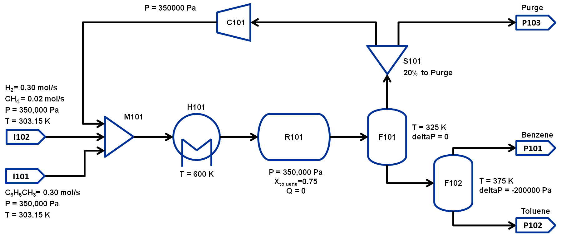
The flowsheet that we will be using for this module is shown below with the stream conditions. We will be processing toluene and hydrogen to produce at least 370 TPY of benzene. As shown in the flowsheet, there are two flash tanks, F101 to separate out the non-condensibles and F102 to further separate the benzene-toluene mixture to improve the benzene purity. Note that typically a distillation column is required to obtain high purity benzene but that is beyond the scope of this workshop. The non-condensibles separated out in F101 will be partially recycled back to M101 and the rest will be either purged or combusted for power generation.We will assume ideal gas for this flowsheet. The properties required for this module are available in the same directory:

hda_ideal_VLE.py
hda_reaction.py

The state variables chosen for the property package are flows of component by phase, temperature and pressure. The components considered are: toluene, hydrogen, benzene and methane. Therefore, every stream has 8 flow variables, 1 temperature and 1 pressure variable.

Importing required pyomo and idaes components#

To construct a flowsheet, we will need several components from the pyomo and idaes package. Let us first import the following components from Pyomo:

Constraint (to write constraints)
Var (to declare variables)
ConcreteModel (to create the concrete model object)
Expression (to evaluate values as a function of variables defined in the model)
Objective (to define an objective function for optimization)
SolverFactory (to solve the problem)
TransformationFactory (to apply certain transformations)
Arc (to connect two unit models)
SequentialDecomposition (to initialize the flowsheet in a sequential mode)

For further details on these components, please refer to the pyomo documentation: https://pyomo.readthedocs.io/en/stable/

from pyomo.environ import (
    Constraint,
    Var,
    ConcreteModel,
    Expression,
    Objective,
    SolverFactory,
    TransformationFactory,
    value,
)
from pyomo.network import Arc, SequentialDecomposition

From idaes, we will be needing the FlowsheetBlock and the following unit models:

Mixer
Heater
StoichiometricReactor
Flash
Separator (splitter)
PressureChanger

from idaes.core import FlowsheetBlock

from idaes.models.unit_models import (
    PressureChanger,
    Mixer,
    Separator as Splitter,
    Heater,
    StoichiometricReactor,
)

Inline Exercise: Now, import the remaining unit models highlighted in blue above and run the cell using `Shift+Enter` after typing in the code.

# Todo: import flash model from idaes.models.unit_models
from idaes.models.unit_models import Flash

We will also be needing some utility tools to put together the flowsheet and calculate the degrees of freedom.

from idaes.models.unit_models.pressure_changer import ThermodynamicAssumption
from idaes.core.util.model_statistics import degrees_of_freedom

# Import idaes logger to set output levels
import idaes.logger as idaeslog

Importing required thermo and reaction package#

The final set of imports are to import the thermo and reaction package for the HDA process. We have created a custom thermo package that assumes Ideal Gas with support for VLE.

The reaction package here is very simple as we will be using only a StochiometricReactor and the reaction package consists of the stochiometric coefficients for the reaction and the parameter for the heat of reaction.

Let us import the following modules and they are in the same directory as this jupyter notebook:

hda_ideal_VLE as thermo_props
hda_reaction as reaction_props

from idaes_examples.mod.hda import hda_ideal_VLE as thermo_props
from idaes_examples.mod.hda import hda_reaction as reaction_props

Constructing the Flowsheet#

We have now imported all the components, unit models, and property modules we need to construct a flowsheet. Let us create a ConcreteModel and add the flowsheet block as we did in module 1.

m = ConcreteModel()
m.fs = FlowsheetBlock(dynamic=False)

We now need to add the property packages to the flowsheet. Unlike Module 1, where we only had a thermo property package, for this flowsheet we will also need to add a reaction property package.

m.fs.thermo_params = thermo_props.HDAParameterBlock()
m.fs.reaction_params = reaction_props.HDAReactionParameterBlock(
    property_package=m.fs.thermo_params
)

WARNING: Params with units must be mutable.  Converting Param
'fs.thermo_params.pressure_crit' to mutable.

WARNING: Params with units must be mutable.  Converting Param
'fs.thermo_params.temperature_crit' to mutable.

WARNING: Params with units must be mutable.  Converting Param
'fs.thermo_params.mw_comp' to mutable.

WARNING: Params with units must be mutable.  Converting Param
'fs.thermo_params.dens_liq_param_1' to mutable.

WARNING: Params with units must be mutable.  Converting Param
'fs.thermo_params.dens_liq_param_2' to mutable.

WARNING: Params with units must be mutable.  Converting Param
'fs.thermo_params.dens_liq_param_3' to mutable.

WARNING: Params with units must be mutable.  Converting Param
'fs.thermo_params.dens_liq_param_4' to mutable.

WARNING: Params with units must be mutable.  Converting Param
'fs.thermo_params.temperature_boil' to mutable.

WARNING: Params with units must be mutable.  Converting Param
'fs.thermo_params.cp_ig_1' to mutable.

WARNING: Params with units must be mutable.  Converting Param
'fs.thermo_params.cp_ig_2' to mutable.

WARNING: Params with units must be mutable.  Converting Param
'fs.thermo_params.cp_ig_3' to mutable.

WARNING: Params with units must be mutable.  Converting Param
'fs.thermo_params.cp_ig_4' to mutable.

WARNING: Params with units must be mutable.  Converting Param
'fs.thermo_params.cp_ig_5' to mutable.

WARNING: Params with units must be mutable.  Converting Param
'fs.thermo_params.pressure_sat_coeff_A' to mutable.

WARNING: Params with units must be mutable.  Converting Param
'fs.thermo_params.pressure_sat_coeff_B' to mutable.

WARNING: Params with units must be mutable.  Converting Param
'fs.thermo_params.pressure_sat_coeff_C' to mutable.

WARNING: Params with units must be mutable.  Converting Param
'fs.thermo_params.dh_vap' to mutable.

Adding Unit Models#

Let us start adding the unit models we have imported to the flowsheet. Here, we are adding the Mixer (assigned a name M101) and a Heater (assigned a name H101). Note that, all unit models need to be given a property package argument. In addition to that, there are several arguments depending on the unit model, please refer to the documentation for more details (https://idaes-pse.readthedocs.io/en/stable/reference_guides/model_libraries/generic/unit_models/index.html). For example, the Mixer unit model here is given a list consisting of names to the three inlets.

m.fs.M101 = Mixer(
    property_package=m.fs.thermo_params,
    inlet_list=["toluene_feed", "hydrogen_feed", "vapor_recycle"],
)

m.fs.H101 = Heater(
    property_package=m.fs.thermo_params,
    has_pressure_change=False,
    has_phase_equilibrium=True,
)

Inline Exercise: Let us now add the StoichiometricReactor(assign the name R101) and pass the following arguments:

"property_package": m.fs.thermo_params
"reaction_package": m.fs.reaction_params
"has_heat_of_reaction": True
"has_heat_transfer": True
"has_pressure_change": False

# Todo: Add reactor with the specifications above
m.fs.R101 = StoichiometricReactor(
    property_package=m.fs.thermo_params,
    reaction_package=m.fs.reaction_params,
    has_heat_of_reaction=True,
    has_heat_transfer=True,
    has_pressure_change=False,
)

Let us now add the Flash(assign the name F101) and pass the following arguments:

”property_package”: m.fs.thermo_params
”has_heat_transfer”: True
”has_pressure_change”: False

m.fs.F101 = Flash(
    property_package=m.fs.thermo_params,
    has_heat_transfer=True,
    has_pressure_change=True,
)

Let us now add the Splitter(S101), PressureChanger(C101) and the second Flash(F102).

m.fs.S101 = Splitter(
    property_package=m.fs.thermo_params,
    ideal_separation=False,
    outlet_list=["purge", "recycle"],
)


m.fs.C101 = PressureChanger(
    property_package=m.fs.thermo_params,
    compressor=True,
    thermodynamic_assumption=ThermodynamicAssumption.isothermal,
)

m.fs.F102 = Flash(
    property_package=m.fs.thermo_params,
    has_heat_transfer=True,
    has_pressure_change=True,
)

Connecting Unit Models using Arcs#

We have now added all the unit models we need to the flowsheet. However, we have not yet specified how the units are to be connected. To do this, we will be using the Arc which is a pyomo component that takes in two arguments: source and destination. Let us connect the outlet of the mixer(M101) to the inlet of the heater(H101).

m.fs.s03 = Arc(source=m.fs.M101.outlet, destination=m.fs.H101.inlet)

Inline Exercise: Now, connect the H101 outlet to the R101 inlet using the cell above as a guide.

# Todo: Connect the H101 outlet to R101 inlet
m.fs.s04 = Arc(source=m.fs.H101.outlet, destination=m.fs.R101.inlet)

We will now be connecting the rest of the flowsheet as shown below. Notice how the outlet names are different for the flash tanks F101 and F102 as they have a vapor and a liquid outlet.

m.fs.s05 = Arc(source=m.fs.R101.outlet, destination=m.fs.F101.inlet)
m.fs.s06 = Arc(source=m.fs.F101.vap_outlet, destination=m.fs.S101.inlet)
m.fs.s08 = Arc(source=m.fs.S101.recycle, destination=m.fs.C101.inlet)
m.fs.s09 = Arc(source=m.fs.C101.outlet, destination=m.fs.M101.vapor_recycle)
m.fs.s10 = Arc(source=m.fs.F101.liq_outlet, destination=m.fs.F102.inlet)

We have now connected the unit model block using the arcs. However, each of these arcs link to ports on the two unit models that are connected. In this case, the ports consist of the state variables that need to be linked between the unit models. Pyomo provides a convenient method to write these equality constraints for us between two ports and this is done as follows:

TransformationFactory("network.expand_arcs").apply_to(m)

Adding expressions to compute purity and operating costs#

In this section, we will add a few Expressions that allows us to evaluate the performance. Expressions provide a convenient way of calculating certain values that are a function of the variables defined in the model. For more details on Expressions, please refer to: https://pyomo.readthedocs.io/en/stable/pyomo_modeling_components/Expressions.html

For this flowsheet, we are interested in computing the purity of the product Benzene stream (i.e. the mole fraction) and the operating cost which is a sum of the cooling and heating cost.

Let us first add an Expression to compute the mole fraction of benzene in the vap_outlet of F102 which is our product stream. Please note that the var flow_mol_phase_comp has the index - [time, phase, component]. As this is a steady-state flowsheet, the time index by default is 0. The valid phases are [“Liq”, “Vap”]. Similarly the valid component list is [“benzene”, “toluene”, “hydrogen”, “methane”].

m.fs.purity = Expression(
    expr=m.fs.F102.vap_outlet.flow_mol_phase_comp[0, "Vap", "benzene"]
    / (
        m.fs.F102.vap_outlet.flow_mol_phase_comp[0, "Vap", "benzene"]
        + m.fs.F102.vap_outlet.flow_mol_phase_comp[0, "Vap", "toluene"]
    )
)

Now, let us add an expression to compute the cooling cost assuming a cost of 0.212E-4 $/kW. Note that cooling utility is required for the reactor (R101) and the first flash (F101).

m.fs.cooling_cost = Expression(
    expr=0.212e-7 * (-m.fs.F101.heat_duty[0]) + 0.212e-7 * (-m.fs.R101.heat_duty[0])
)

Now, let us add an expression to compute the heating cost assuming the utility cost as follows:

2.2E-4 dollars/kW for H101
1.9E-4 dollars/kW for F102

Note that the heat duty is in units of watt (J/s).

m.fs.heating_cost = Expression(
    expr=2.2e-7 * m.fs.H101.heat_duty[0] + 1.9e-7 * m.fs.F102.heat_duty[0]
)

Let us now add an expression to compute the total operating cost per year which is basically the sum of the cooling and heating cost we defined above.

m.fs.operating_cost = Expression(
    expr=(3600 * 24 * 365 * (m.fs.heating_cost + m.fs.cooling_cost))
)

Fixing feed conditions#

Let us first check how many degrees of freedom exist for this flowsheet using the degrees_of_freedom tool we imported earlier.

print(degrees_of_freedom(m))

We will now be fixing the toluene feed stream to the conditions shown in the flowsheet above. Please note that though this is a pure toluene feed, the remaining components are still assigned a very small non-zero value to help with convergence and initializing.

m.fs.M101.toluene_feed.flow_mol_phase_comp[0, "Vap", "benzene"].fix(1e-5)
m.fs.M101.toluene_feed.flow_mol_phase_comp[0, "Vap", "toluene"].fix(1e-5)
m.fs.M101.toluene_feed.flow_mol_phase_comp[0, "Vap", "hydrogen"].fix(1e-5)
m.fs.M101.toluene_feed.flow_mol_phase_comp[0, "Vap", "methane"].fix(1e-5)
m.fs.M101.toluene_feed.flow_mol_phase_comp[0, "Liq", "benzene"].fix(1e-5)
m.fs.M101.toluene_feed.flow_mol_phase_comp[0, "Liq", "toluene"].fix(0.30)
m.fs.M101.toluene_feed.flow_mol_phase_comp[0, "Liq", "hydrogen"].fix(1e-5)
m.fs.M101.toluene_feed.flow_mol_phase_comp[0, "Liq", "methane"].fix(1e-5)
m.fs.M101.toluene_feed.temperature.fix(303.2)
m.fs.M101.toluene_feed.pressure.fix(350000)

Similarly, let us fix the hydrogen feed to the following conditions in the next cell:

F_H2 = 0.30 mol/s
F_CH4 = 0.02 mol/s
Remaining components = 1e-5 mol/s
T = 303.2 K
P = 350000 Pa

m.fs.M101.hydrogen_feed.flow_mol_phase_comp[0, "Vap", "benzene"].fix(1e-5)
m.fs.M101.hydrogen_feed.flow_mol_phase_comp[0, "Vap", "toluene"].fix(1e-5)
m.fs.M101.hydrogen_feed.flow_mol_phase_comp[0, "Vap", "hydrogen"].fix(0.30)
m.fs.M101.hydrogen_feed.flow_mol_phase_comp[0, "Vap", "methane"].fix(0.02)
m.fs.M101.hydrogen_feed.flow_mol_phase_comp[0, "Liq", "benzene"].fix(1e-5)
m.fs.M101.hydrogen_feed.flow_mol_phase_comp[0, "Liq", "toluene"].fix(1e-5)
m.fs.M101.hydrogen_feed.flow_mol_phase_comp[0, "Liq", "hydrogen"].fix(1e-5)
m.fs.M101.hydrogen_feed.flow_mol_phase_comp[0, "Liq", "methane"].fix(1e-5)
m.fs.M101.hydrogen_feed.temperature.fix(303.2)
m.fs.M101.hydrogen_feed.pressure.fix(350000)

Fixing unit model specifications#

Now that we have fixed our inlet feed conditions, we will now be fixing the operating conditions for the unit models in the flowsheet. Let us set set the H101 outlet temperature to 600 K.

m.fs.H101.outlet.temperature.fix(600)

For the StoichiometricReactor, we have to define the conversion in terms of toluene. This requires us to create a new variable for specifying the conversion and adding a Constraint that defines the conversion with respect to toluene. The second degree of freedom for the reactor is to define the heat duty. In this case, let us assume the reactor to be adiabatic i.e. Q = 0.

m.fs.R101.conversion = Var(initialize=0.75, bounds=(0, 1))

m.fs.R101.conv_constraint = Constraint(
    expr=m.fs.R101.conversion * m.fs.R101.inlet.flow_mol_phase_comp[0, "Vap", "toluene"]
    == (
        m.fs.R101.inlet.flow_mol_phase_comp[0, "Vap", "toluene"]
        - m.fs.R101.outlet.flow_mol_phase_comp[0, "Vap", "toluene"]
    )
)

m.fs.R101.conversion.fix(0.75)
m.fs.R101.heat_duty.fix(0)

The Flash conditions for F101 can be set as follows.

m.fs.F101.vap_outlet.temperature.fix(325.0)
m.fs.F101.deltaP.fix(0)

Inline Exercise: Set the conditions for Flash F102 to the following conditions:

T = 375 K
deltaP = -200000

Use Shift+Enter to run the cell once you have typed in your code.

m.fs.F102.vap_outlet.temperature.fix(375)
m.fs.F102.deltaP.fix(-200000)

Let us fix the purge split fraction to 20% and the outlet pressure of the compressor is set to 350000 Pa.

m.fs.S101.split_fraction[0, "purge"].fix(0.2)
m.fs.C101.outlet.pressure.fix(350000)

Inline Exercise: We have now defined all the feed conditions and the inputs required for the unit models. The system should now have 0 degrees of freedom i.e. should be a square problem. Please check that the degrees of freedom is 0.

Use Shift+Enter to run the cell once you have typed in your code.

print(degrees_of_freedom(m))

Initialization#

This section will demonstrate how to use the built-in sequential decomposition tool to initialize our flowsheet.

Let us first create an object for the SequentialDecomposition and specify our options for this.

seq = SequentialDecomposition()
seq.options.select_tear_method = "heuristic"
seq.options.tear_method = "Wegstein"
seq.options.iterLim = 3

# Using the SD tool
G = seq.create_graph(m)
heuristic_tear_set = seq.tear_set_arcs(G, method="heuristic")
order = seq.calculation_order(G)

Which is the tear stream? Display tear set and order

for o in heuristic_tear_set:
    print(o.name)

fs.s03

What sequence did the SD tool determine to solve this flowsheet with the least number of tears?

for o in order:
    print(o[0].name)

fs.H101
fs.R101
fs.F101
fs.S101
fs.C101
fs.M101

The SequentialDecomposition tool has determined that the tear stream is the mixer outlet. We will need to provide a reasonable guess for this.

tear_guesses = {
    "flow_mol_phase_comp": {
        (0, "Vap", "benzene"): 1e-5,
        (0, "Vap", "toluene"): 1e-5,
        (0, "Vap", "hydrogen"): 0.30,
        (0, "Vap", "methane"): 0.02,
        (0, "Liq", "benzene"): 1e-5,
        (0, "Liq", "toluene"): 0.30,
        (0, "Liq", "hydrogen"): 1e-5,
        (0, "Liq", "methane"): 1e-5,
    },
    "temperature": {0: 303},
    "pressure": {0: 350000},
}

# Pass the tear_guess to the SD tool
seq.set_guesses_for(m.fs.H101.inlet, tear_guesses)

Next, we need to tell the tool how to initialize a particular unit. We will be writing a python function which takes in a “unit” and calls the initialize method on that unit.

def function(unit):
    unit.initialize(outlvl=idaeslog.INFO)

We are now ready to initialize our flowsheet in a sequential mode. Note that we specifically set the iteration limit to be 5 as we are trying to use this tool only to get a good set of initial values such that IPOPT can then take over and solve this flowsheet for us.

seq.run(m, function)

2024-05-09 18:38:52 [INFO] idaes.init.fs.H101.control_volume: Initialization Complete

---------------------------------------------------------------------------
ApplicationError                          Traceback (most recent call last)
Cell In[36], line 1
----> 1 seq.run(m, function)

File ~/checkouts/readthedocs.org/user_builds/idaes-examples/envs/latest/lib/python3.8/site-packages/pyomo/network/decomposition.py:296, in SequentialDecomposition.run(self, model, function)
    293 self.cache.clear()
    295 try:
--> 296     return self._run_impl(model, function)
    297 finally:
    298     # Cleanup
    299     self.cache.clear()

File ~/checkouts/readthedocs.org/user_builds/idaes-examples/envs/latest/lib/python3.8/site-packages/pyomo/network/decomposition.py:317, in SequentialDecomposition._run_impl(self, model, function)
    315     logger.info("Starting first pass run of network")
    316     order = self.calculation_order(G)
--> 317     self.run_order(G, order, function, tset, use_guesses=True)
    319 if not self.options["solve_tears"] or not len(tset):
    320     # Not solving tears, we're done
    321     end = time.time()

File ~/checkouts/readthedocs.org/user_builds/idaes-examples/envs/latest/lib/python3.8/site-packages/pyomo/network/decomposition.py:407, in SequentialDecomposition.run_order(self, G, order, function, ignore, use_guesses)
    404         self.load_guesses(guesses, port, fixed_ins)
    405     self.load_values(port, default, fixed_ins, use_guesses)
--> 407 function(unit)
    409 # free the inputs that were not already fixed
    410 for var in fixed_ins:

Cell In[35], line 2, in function(unit)
      1 def function(unit):
----> 2     unit.initialize(outlvl=idaeslog.INFO)

File ~/checkouts/readthedocs.org/user_builds/idaes-examples/envs/latest/lib/python3.8/site-packages/idaes/core/base/unit_model.py:540, in UnitModelBlockData.initialize(blk, *args, **kwargs)
    537     c.deactivate()
    539 # Remember to collect flags for fixed vars
--> 540 flags = blk.initialize_build(*args, **kwargs)
    542 # If costing block exists, activate and initialize
    543 for c in init_order:

File ~/checkouts/readthedocs.org/user_builds/idaes-examples/envs/latest/lib/python3.8/site-packages/idaes/core/base/unit_model.py:601, in UnitModelBlockData.initialize_build(blk, state_args, outlvl, solver, optarg)
    598 # ---------------------------------------------------------------------
    599 # Solve unit
    600 with idaeslog.solver_log(solve_log, idaeslog.DEBUG) as slc:
--> 601     results = opt.solve(blk, tee=slc.tee)
    603 init_log.info_high(
    604     "Initialization Step 2 {}.".format(idaeslog.condition(results))
    605 )
    607 # ---------------------------------------------------------------------
    608 # Release Inlet state

File ~/checkouts/readthedocs.org/user_builds/idaes-examples/envs/latest/lib/python3.8/site-packages/pyomo/opt/base/solvers.py:534, in OptSolver.solve(self, *args, **kwds)
    531 def solve(self, *args, **kwds):
    532     """Solve the problem"""
--> 534     self.available(exception_flag=True)
    535     #
    536     # If the inputs are models, then validate that they have been
    537     # constructed! Collect suffix names to try and import from solution.
    538     #
    539     from pyomo.core.base.block import BlockData

File ~/checkouts/readthedocs.org/user_builds/idaes-examples/envs/latest/lib/python3.8/site-packages/pyomo/opt/solver/shellcmd.py:140, in SystemCallSolver.available(self, exception_flag)
    138     if exception_flag:
    139         msg = "No executable found for solver '%s'"
--> 140         raise ApplicationError(msg % self.name)
    141     return False
    142 return True

ApplicationError: No executable found for solver 'ipopt'

Inline Exercise: We have now initialized the flowsheet. Let us run the flowsheet in a simulation mode to look at the results. To do this, complete the last line of code where we pass the model to the solver. You will need to type the following:

results = solver.solve(m, tee=True)

Use Shift+Enter to run the cell once you have typed in your code.

# Create the solver object
from idaes.core.solvers import get_solver

solver = get_solver()

# Solve the model
results = solver.solve(m, tee=True)

Ipopt 3.13.2: nlp_scaling_method=gradient-based
tol=1e-06
max_iter=200


******************************************************************************
This program contains Ipopt, a library for large-scale nonlinear optimization.
 Ipopt is released as open source code under the Eclipse Public License (EPL).
         For more information visit http://projects.coin-or.org/Ipopt

This version of Ipopt was compiled from source code available at
    https://github.com/IDAES/Ipopt as part of the Institute for the Design of
    Advanced Energy Systems Process Systems Engineering Framework (IDAES PSE
    Framework) Copyright (c) 2018-2019. See https://github.com/IDAES/idaes-pse.

This version of Ipopt was compiled using HSL, a collection of Fortran codes
    for large-scale scientific computation.  All technical papers, sales and
    publicity material resulting from use of the HSL codes within IPOPT must
    contain the following acknowledgement:
        HSL, a collection of Fortran codes for large-scale scientific
        computation. See http://www.hsl.rl.ac.uk.
******************************************************************************

This is Ipopt version 3.13.2, running with linear solver ma27.

Number of nonzeros in equality constraint Jacobian...:     1031
Number of nonzeros in inequality constraint Jacobian.:        0
Number of nonzeros in Lagrangian Hessian.............:      934

Total number of variables............................:      340
                     variables with only lower bounds:        0
                variables with lower and upper bounds:      146
                     variables with only upper bounds:        0
Total number of equality constraints.................:      340
Total number of inequality constraints...............:        0
        inequality constraints with only lower bounds:        0
   inequality constraints with lower and upper bounds:        0
        inequality constraints with only upper bounds:        0

iter    objective    inf_pr   inf_du lg(mu)  ||d||  lg(rg) alpha_du alpha_pr  ls
   0  0.0000000e+00 6.60e+04 0.00e+00  -1.0 0.00e+00    -  0.00e+00 0.00e+00   0
   1  0.0000000e+00 8.69e+03 1.42e+03  -1.0 2.00e+04    -  9.71e-01 4.67e-01H  1
   2  0.0000000e+00 3.05e+03 1.56e+03  -1.0 1.60e+04    -  9.79e-01 4.90e-01h  1
   3  0.0000000e+00 1.58e+03 1.55e+05  -1.0 1.41e+04    -  9.90e-01 4.99e-01h  1
   4  0.0000000e+00 5.49e+02 8.87e+08  -1.0 8.43e+03    -  1.00e+00 9.57e-01h  1
   5  0.0000000e+00 4.25e+03 2.87e+10  -1.0 8.02e+02    -  1.00e+00 9.90e-01h  1
   6  0.0000000e+00 2.25e+03 1.51e+10  -1.0 8.39e+00    -  1.00e+00 1.00e+00h  1
   7  0.0000000e+00 2.27e+01 1.40e+08  -1.0 2.45e-03    -  1.00e+00 1.00e+00f  1
   8  0.0000000e+00 2.45e-03 1.23e+04  -1.0 2.38e-05    -  1.00e+00 1.00e+00h  1
   9  0.0000000e+00 7.45e-09 3.06e-01  -2.5 9.06e-08    -  1.00e+00 1.00e+00h  1
Cannot recompute multipliers for feasibility problem.  Error in eq_mult_calculator

Number of Iterations....: 9

                                   (scaled)                 (unscaled)
Objective...............:   0.0000000000000000e+00    0.0000000000000000e+00
Dual infeasibility......:   2.8284422320850682e+05    2.8284422320850682e+05
Constraint violation....:   2.9103830456733704e-11    7.4505805969238281e-09
Complementarity.........:   0.0000000000000000e+00    0.0000000000000000e+00
Overall NLP error.......:   2.9103830456733704e-11    2.8284422320850682e+05


Number of objective function evaluations             = 11
Number of objective gradient evaluations             = 10
Number of equality constraint evaluations            = 11
Number of inequality constraint evaluations          = 0
Number of equality constraint Jacobian evaluations   = 10
Number of inequality constraint Jacobian evaluations = 0
Number of Lagrangian Hessian evaluations             = 9
Total CPU secs in IPOPT (w/o function evaluations)   =      0.004
Total CPU secs in NLP function evaluations           =      0.000

EXIT: Optimal Solution Found.

Analyze the results of the square problem#

What is the total operating cost?

print("operating cost = $", value(m.fs.operating_cost))

operating cost = $ 419122.3387677983

For this operating cost, what is the amount of benzene we are able to produce and what purity we are able to achieve?

m.fs.F102.report()

print()
print("benzene purity = ", value(m.fs.purity))

====================================================================================
Unit : fs.F102                                                             Time: 0.0
------------------------------------------------------------------------------------
    Unit Performance

    Variables: 

    Key             : Value       : Units  : Fixed : Bounds
          Heat Duty :      7352.5 :   watt : False : (None, None)
    Pressure Change : -2.0000e+05 : pascal :  True : (None, None)

------------------------------------------------------------------------------------
    Stream Table
                                                Units         Inlet    Vapor Outlet  Liquid Outlet
    flow_mol_phase_comp ('Liq', 'benzene')   mole / second    0.20460   1.0000e-08      0.062620  
    flow_mol_phase_comp ('Liq', 'toluene')   mole / second   0.062520   1.0000e-08      0.032257  
    flow_mol_phase_comp ('Liq', 'methane')   mole / second 2.6712e-07   1.0000e-08    9.4877e-08  
    flow_mol_phase_comp ('Liq', 'hydrogen')  mole / second 2.6712e-07   1.0000e-08    9.4877e-08  
    flow_mol_phase_comp ('Vap', 'benzene')   mole / second 1.0000e-08      0.14198    1.0000e-08  
    flow_mol_phase_comp ('Vap', 'toluene')   mole / second 1.0000e-08     0.030264    1.0000e-08  
    flow_mol_phase_comp ('Vap', 'methane')   mole / second 1.0000e-08   1.8224e-07    1.0000e-08  
    flow_mol_phase_comp ('Vap', 'hydrogen')  mole / second 1.0000e-08   1.8224e-07    1.0000e-08  
    temperature                                     kelvin     325.00       375.00        375.00  
    pressure                                        pascal 3.5000e+05   1.5000e+05    1.5000e+05  
====================================================================================

benzene purity =  0.8242962943918918

Next, let’s look at how much benzene we are losing with the light gases out of F101. IDAES has tools for creating stream tables based on the Arcs and/or Ports in a flowsheet. Let us create and print a simple stream table showing the stream leaving the reactor and the vapor stream from F101.

Inline Exercise: How much benzene are we losing in the F101 vapor outlet stream?

from idaes.core.util.tables import (
    create_stream_table_dataframe,
    stream_table_dataframe_to_string,
)

st = create_stream_table_dataframe({"Reactor": m.fs.s05, "Light Gases": m.fs.s06})
print(stream_table_dataframe_to_string(st))

                                            Units        Reactor   Light Gases
flow_mol_phase_comp ('Liq', 'benzene')   mole / second 1.2993e-07  1.0000e-08 
flow_mol_phase_comp ('Liq', 'toluene')   mole / second 8.4147e-07  1.0000e-08 
flow_mol_phase_comp ('Liq', 'methane')   mole / second 1.0000e-12  1.0000e-08 
flow_mol_phase_comp ('Liq', 'hydrogen')  mole / second 1.0000e-12  1.0000e-08 
flow_mol_phase_comp ('Vap', 'benzene')   mole / second    0.35374     0.14915 
flow_mol_phase_comp ('Vap', 'toluene')   mole / second   0.078129    0.015610 
flow_mol_phase_comp ('Vap', 'methane')   mole / second     1.2721      1.2721 
flow_mol_phase_comp ('Vap', 'hydrogen')  mole / second    0.32821     0.32821 
temperature                                     kelvin     771.85      325.00 
pressure                                        pascal 3.5000e+05  3.5000e+05 

Inline Exercise: You can query additional variables here if you like.

Use Shift+Enter to run the cell once you have typed in your code.

Optimization#

We saw from the results above that the total operating cost for the base case was $419,122 per year. We are producing 0.142 mol/s of benzene at a purity of 82%. However, we are losing around 42% of benzene in F101 vapor outlet stream.

Let us try to minimize this cost such that:

we are producing at least 0.15 mol/s of benzene in F102 vapor outlet i.e. our product stream
purity of benzene i.e. the mole fraction of benzene in F102 vapor outlet is at least 80%
restricting the benzene loss in F101 vapor outlet to less than 20%

For this problem, our decision variables are as follows:

H101 outlet temperature
R101 cooling duty provided
F101 outlet temperature
F102 outlet temperature
F102 deltaP in the flash tank

Let us declare our objective function for this problem.

m.fs.objective = Objective(expr=m.fs.operating_cost)

Now, we need to unfix the decision variables as we had solved a square problem (degrees of freedom = 0) until now.

m.fs.H101.outlet.temperature.unfix()
m.fs.R101.heat_duty.unfix()
m.fs.F101.vap_outlet.temperature.unfix()
m.fs.F102.vap_outlet.temperature.unfix()

Inline Exercise: Let us now unfix the remaining variable which is F102 pressure drop (F102.deltaP)

Use Shift+Enter to run the cell once you have typed in your code.

# Todo: Unfix deltaP for F102
m.fs.F102.deltaP.unfix()

Next, we need to set bounds on these decision variables to values shown below:

H101 outlet temperature [500, 600] K
R101 outlet temperature [600, 800] K
F101 outlet temperature [298, 450] K
F102 outlet temperature [298, 450] K
F102 outlet pressure [105000, 110000] Pa

Let us first set the variable bound for the H101 outlet temperature as shown below:

m.fs.H101.outlet.temperature[0].setlb(500)
m.fs.H101.outlet.temperature[0].setub(600)

Inline Exercise: Now, set the variable bound for the R101 outlet temperature.

Use Shift+Enter to run the cell once you have typed in your code.

# Todo: Set the bounds for reactor outlet temperature
m.fs.R101.outlet.temperature[0].setlb(600)
m.fs.R101.outlet.temperature[0].setub(800)

Let us fix the bounds for the rest of the decision variables.

m.fs.F101.vap_outlet.temperature[0].setlb(298.0)
m.fs.F101.vap_outlet.temperature[0].setub(450.0)
m.fs.F102.vap_outlet.temperature[0].setlb(298.0)
m.fs.F102.vap_outlet.temperature[0].setub(450.0)
m.fs.F102.vap_outlet.pressure[0].setlb(105000)
m.fs.F102.vap_outlet.pressure[0].setub(110000)

Now, the only things left to define are our constraints on overhead loss in F101, product flow rate and purity in F102. Let us first look at defining a constraint for the overhead loss in F101 where we are restricting the benzene leaving the vapor stream to less than 20 % of the benzene available in the reactor outlet.

m.fs.overhead_loss = Constraint(
    expr=m.fs.F101.vap_outlet.flow_mol_phase_comp[0, "Vap", "benzene"]
    <= 0.20 * m.fs.R101.outlet.flow_mol_phase_comp[0, "Vap", "benzene"]
)

Inline Exercise: Now, add the constraint such that we are producing at least 0.15 mol/s of benzene in the product stream which is the vapor outlet of F102. Let us name this constraint as m.fs.product_flow.

Use Shift+Enter to run the cell once you have typed in your code.

# Todo: Add minimum product flow constraint
m.fs.product_flow = Constraint(
    expr=m.fs.F102.vap_outlet.flow_mol_phase_comp[0, "Vap", "benzene"] >= 0.15
)

Let us add the final constraint on product purity or the mole fraction of benzene in the product stream such that it is at least greater than 80%.

m.fs.product_purity = Constraint(expr=m.fs.purity >= 0.80)

We have now defined the optimization problem and we are now ready to solve this problem.

results = solver.solve(m, tee=True)

Ipopt 3.13.2: nlp_scaling_method=gradient-based
tol=1e-06
max_iter=200

******************************************************************************
This program contains Ipopt, a library for large-scale nonlinear optimization.
 Ipopt is released as open source code under the Eclipse Public License (EPL).
         For more information visit http://projects.coin-or.org/Ipopt

This version of Ipopt was compiled from source code available at
    https://github.com/IDAES/Ipopt as part of the Institute for the Design of
    Advanced Energy Systems Process Systems Engineering Framework (IDAES PSE
    Framework) Copyright (c) 2018-2019. See https://github.com/IDAES/idaes-pse.

This version of Ipopt was compiled using HSL, a collection of Fortran codes
    for large-scale scientific computation.  All technical papers, sales and
    publicity material resulting from use of the HSL codes within IPOPT must
    contain the following acknowledgement:
        HSL, a collection of Fortran codes for large-scale scientific
        computation. See http://www.hsl.rl.ac.uk.
******************************************************************************

This is Ipopt version 3.13.2, running with linear solver ma27.

Number of nonzeros in equality constraint Jacobian...:     1057
Number of nonzeros in inequality constraint Jacobian.:        5
Number of nonzeros in Lagrangian Hessian.............:      937

Total number of variables............................:      345
                     variables with only lower bounds:        0
                variables with lower and upper bounds:      149
                     variables with only upper bounds:        0
Total number of equality constraints.................:      340
Total number of inequality constraints...............:        3
        inequality constraints with only lower bounds:        2
   inequality constraints with lower and upper bounds:        0
        inequality constraints with only upper bounds:        1

iter    objective    inf_pr   inf_du lg(mu)  ||d||  lg(rg) alpha_du alpha_pr  ls
   0  4.1912234e+05 2.99e+05 6.94e+00  -1.0 0.00e+00    -  0.00e+00 0.00e+00   0
   1  4.1628385e+05 2.99e+05 6.94e+00  -1.0 4.82e+09    -  1.80e-05 5.83e-06f  1
   2  4.1616723e+05 2.99e+05 1.59e+02  -1.0 1.46e+09    -  5.83e-04 1.47e-05f  1
   3  4.0789953e+05 2.94e+05 4.83e+02  -1.0 1.36e+09    -  2.64e-04 9.30e-04f  1
   4  2.9668590e+05 2.83e+06 6.97e+02  -1.0 4.80e+08    -  7.26e-05 1.50e-03f  1
   5  2.9555461e+05 2.83e+06 4.95e+04  -1.0 1.90e+08    -  1.88e-01 1.04e-03f  1
   6  2.9451022e+05 2.73e+06 4.60e+05  -1.0 4.43e+07    -  1.87e-01 3.43e-02f  1
   7  2.9628497e+05 2.13e+06 4.43e+05  -1.0 1.48e+07    -  7.40e-02 2.18e-01h  1
   8  2.9632658e+05 2.13e+06 4.41e+05  -1.0 5.91e+06    -  6.37e-01 3.36e-03h  1
   9  2.9642679e+05 2.11e+06 4.39e+05  -1.0 6.54e+06    -  7.26e-01 7.12e-03h  1
iter    objective    inf_pr   inf_du lg(mu)  ||d||  lg(rg) alpha_du alpha_pr  ls
  10  2.9954735e+05 1.64e+06 4.13e+05  -1.0 6.57e+06    -  3.57e-02 2.24e-01h  1
  11  3.0435085e+05 9.50e+05 6.95e+05  -1.0 5.56e+06    -  9.46e-01 4.20e-01h  1
  12  3.0895827e+05 3.69e+05 1.22e+07  -1.0 4.03e+06    -  9.90e-01 6.11e-01h  1
  13  3.1246277e+05 1.42e+06 1.80e+10  -1.0 2.25e+06    -  9.95e-01 9.65e-01h  1
  14  3.1266092e+05 5.66e+05 7.10e+10  -1.0 2.77e+05    -  4.14e-01 6.11e-01h  1
  15  3.1266072e+05 5.65e+05 7.08e+10  -1.0 1.18e+06    -  1.09e-02 2.60e-04h  1
  16  3.1266230e+05 5.58e+05 7.01e+10  -1.0 1.08e+05    -  1.00e+00 1.26e-02h  1
  17  3.1271669e+05 3.14e+05 7.23e+10  -1.0 1.07e+05    -  4.05e-01 4.39e-01h  1
  18  3.1278583e+05 3.89e+03 1.58e+10  -1.0 6.01e+04    -  7.76e-03 9.91e-01h  1
  19  3.1278664e+05 1.57e+03 6.81e+10  -1.0 5.59e+02    -  9.87e-01 1.00e+00h  1
iter    objective    inf_pr   inf_du lg(mu)  ||d||  lg(rg) alpha_du alpha_pr  ls
  20  3.1278678e+05 2.39e+01 1.24e+09  -1.0 1.96e+02    -  1.00e+00 1.00e+00f  1
  21  3.1278674e+05 1.19e+01 6.32e+08  -1.0 1.30e+02    -  1.00e+00 5.00e-01f  2
  22  3.1278674e+05 1.21e-02 9.81e+04  -1.0 2.70e+00    -  1.00e+00 1.00e+00f  1
  23  3.1278642e+05 2.23e-05 2.00e+05  -1.7 1.62e+02    -  1.00e+00 1.00e+00f  1
  24  3.1278642e+05 1.49e-08 2.16e-03  -1.7 6.37e-01    -  1.00e+00 1.00e+00h  1
  25  3.1278634e+05 1.38e-06 1.26e+04  -7.0 4.04e+01    -  1.00e+00 1.00e+00f  1
  26  3.1278634e+05 1.49e-08 7.76e-05  -7.0 6.55e-03    -  1.00e+00 1.00e+00h  1

Number of Iterations....: 26

                                   (scaled)                 (unscaled)
Objective...............:   3.1278633834102686e+05    3.1278633834102686e+05
Dual infeasibility......:   7.7559902882953563e-05    7.7559902882953563e-05
Constraint violation....:   5.8207660913467407e-11    1.4901161193847656e-08
Complementarity.........:   9.0926527280252943e-08    9.0926527280252943e-08
Overall NLP error.......:   6.6903080882730816e-09    7.7559902882953563e-05


Number of objective function evaluations             = 28
Number of objective gradient evaluations             = 27
Number of equality constraint evaluations            = 28
Number of inequality constraint evaluations          = 28
Number of equality constraint Jacobian evaluations   = 27
Number of inequality constraint Jacobian evaluations = 27
Number of Lagrangian Hessian evaluations             = 26
Total CPU secs in IPOPT (w/o function evaluations)   =      0.016
Total CPU secs in NLP function evaluations           =      0.000

EXIT: Optimal Solution Found.

Optimization Results#

Display the results and product specifications

print("operating cost = $", value(m.fs.operating_cost))

print()
print("Product flow rate and purity in F102")

m.fs.F102.report()

print()
print("benzene purity = ", value(m.fs.purity))

print()
print("Overhead loss in F101")
m.fs.F101.report()

operating cost = $ 312786.3383410268

Product flow rate and purity in F102

====================================================================================
Unit : fs.F102                                                             Time: 0.0
------------------------------------------------------------------------------------
    Unit Performance

    Variables: 

    Key             : Value       : Units  : Fixed : Bounds
          Heat Duty :      8377.0 :   watt : False : (None, None)
    Pressure Change : -2.4500e+05 : pascal : False : (None, None)

------------------------------------------------------------------------------------
    Stream Table
                                                Units         Inlet    Vapor Outlet  Liquid Outlet
    flow_mol_phase_comp ('Liq', 'benzene')   mole / second    0.21743   1.0000e-08      0.067425  
    flow_mol_phase_comp ('Liq', 'toluene')   mole / second   0.070695   1.0000e-08      0.037507  
    flow_mol_phase_comp ('Liq', 'methane')   mole / second 2.8812e-07   1.0000e-08    1.0493e-07  
    flow_mol_phase_comp ('Liq', 'hydrogen')  mole / second 2.8812e-07   1.0000e-08    1.0493e-07  
    flow_mol_phase_comp ('Vap', 'benzene')   mole / second 1.0000e-08      0.15000    1.0000e-08  
    flow_mol_phase_comp ('Vap', 'toluene')   mole / second 1.0000e-08     0.033189    1.0000e-08  
    flow_mol_phase_comp ('Vap', 'methane')   mole / second 1.0000e-08   1.9319e-07    1.0000e-08  
    flow_mol_phase_comp ('Vap', 'hydrogen')  mole / second 1.0000e-08   1.9319e-07    1.0000e-08  
    temperature                                     kelvin     301.88       362.93        362.93  
    pressure                                        pascal 3.5000e+05   1.0500e+05    1.0500e+05  
====================================================================================

benzene purity =  0.8188276578112285

Overhead loss in F101

====================================================================================
Unit : fs.F101                                                             Time: 0.0
------------------------------------------------------------------------------------
    Unit Performance

    Variables: 

    Key             : Value   : Units  : Fixed : Bounds
          Heat Duty : -56353. :   watt : False : (None, None)
    Pressure Change :  0.0000 : pascal :  True : (None, None)

------------------------------------------------------------------------------------
    Stream Table
                                                Units         Inlet    Vapor Outlet  Liquid Outlet
    flow_mol_phase_comp ('Liq', 'benzene')   mole / second 4.3534e-08   1.0000e-08       0.21743  
    flow_mol_phase_comp ('Liq', 'toluene')   mole / second 7.5866e-07   1.0000e-08      0.070695  
    flow_mol_phase_comp ('Liq', 'methane')   mole / second 1.0000e-12   1.0000e-08    2.8812e-07  
    flow_mol_phase_comp ('Liq', 'hydrogen')  mole / second 1.0000e-12   1.0000e-08    2.8812e-07  
    flow_mol_phase_comp ('Vap', 'benzene')   mole / second    0.27178     0.054356    1.0000e-08  
    flow_mol_phase_comp ('Vap', 'toluene')   mole / second   0.076085    0.0053908    1.0000e-08  
    flow_mol_phase_comp ('Vap', 'methane')   mole / second     1.2414       1.2414    1.0000e-08  
    flow_mol_phase_comp ('Vap', 'hydrogen')  mole / second    0.35887      0.35887    1.0000e-08  
    temperature                                     kelvin     696.11       301.88        301.88  
    pressure                                        pascal 3.5000e+05   3.5000e+05    3.5000e+05  
====================================================================================

Display optimal values for the decision variables

print("Optimal Values")
print()

print("H101 outlet temperature = ", value(m.fs.H101.outlet.temperature[0]), "K")

print()
print("R101 outlet temperature = ", value(m.fs.R101.outlet.temperature[0]), "K")

print()
print("F101 outlet temperature = ", value(m.fs.F101.vap_outlet.temperature[0]), "K")

print()
print("F102 outlet temperature = ", value(m.fs.F102.vap_outlet.temperature[0]), "K")
print("F102 outlet pressure = ", value(m.fs.F102.vap_outlet.pressure[0]), "Pa")

Optimal Values

H101 outlet temperature =  500.0 K

R101 outlet temperature =  696.1117584980856 K

F101 outlet temperature =  301.8784760569282 K

F102 outlet temperature =  362.93476830548985 K
F102 outlet pressure =  105000.0 Pa

HDA Flowsheet Simulation and Optimization

Contents

HDA Flowsheet Simulation and Optimization#

Learning outcomes#

Problem Statement#

Importing required pyomo and idaes components#

Importing required thermo and reaction package#

Constructing the Flowsheet#

Adding Unit Models#

Connecting Unit Models using Arcs#

Adding expressions to compute purity and operating costs#

Fixing feed conditions#

Fixing unit model specifications#

Initialization#

Analyze the results of the square problem#

Optimization#

Optimization Results#