TSA Adsorption Cycle for Carbon Capture

TSA Adsorption Cycle for Carbon Capture#

Maintainer: Daison Yancy Caballero and Alexander Noring
Author: Daison Yancy Caballero and Alexander Noring
Updated: 2023-11-13

Learning outcomes#

Demonstrate the use of the IDAES fixed bed temperature swing adsorption (TSA) 0D unit model
Initialize the IDAES fixed bed TSA 0D unit model
Simulate the IDAES fixed bed TSA 0D unit model by solving a square problem
Generate and analyze results

Problem Statement#

This Jupyter notebook shows the simulation of a fixed bed TSA cycle for carbon capture by using the fixed bed TSA 0D unit model in IDAES. The fixed bed TSA model consists of a 0D equilibrium-based shortcut model composed of four steps a) heating, b) cooling, c) pressurization, and d) adsorption. Note that the equations in the IDAES fixed bed TSA 0D unit model and the input specifications used in this tutorial for the feed stream have been taken from Joss et al. 2015.

A diagram of the TSA adsorption cycle is given below:#

Step 1: Import Libraries#

Import Pyomo packages#

We will need the following components from the pyomo libraries.

ConcreteModel (to create the Pyomo model that will contain the IDAES flowsheet)
TransformationFactory (to apply certain transformations)
SolverFactory (to set up the solver that will solve the problem)
Constraint (to write constraints)
Var (to declare variables)
Objective (to declare an objective function)
minimize (to minimize an objective function)
value (to return the numerical value of an Pyomo objects such as variables, constraints or expressions)
units (to handle units in Pyomo and IDAES)
check_optimal_termination (this method returns the solution status from solver)

For further details on these components, please refer to the Pyomo documentation:

# python libraries
import os

# pyomo libraries
from pyomo.environ import (
    ConcreteModel,
    TransformationFactory,
    SolverFactory,
    Constraint,
    Var,
    Objective,
    minimize,
    value,
    units,
    check_optimal_termination,
)

Import IDAES core components#

To build, initialize, and solve IDAES flowsheets we will need the following core components/utilities:

FlowsheetBlock (the flowsheet block contains idaes properties, time, and unit models)
degrees_of_freedom (useful for debugging, this method returns the DOF of the model)
FixedBedTSA0D (fixed bed TSA model unit model)
util (some utility functions in IDAES)
idaeslog (it’s used to set output messages like warnings or errors)

For further details on these components, please refer to the IDAES documentation:

# import IDAES core libraries 
from idaes.core import FlowsheetBlock
from idaes.core.util.model_statistics import degrees_of_freedom
import idaes.core.util as iutil
import idaes.logger as idaeslog

# import tsa unit model
from idaes.models_extra.temperature_swing_adsorption import (
    FixedBedTSA0D,
    FixedBedTSA0DInitializer,
    Adsorbent,
)
from idaes.models_extra.temperature_swing_adsorption.util import tsa_summary, plot_tsa_profiles

Step 2: Constructing the Flowsheet#

First, let’s create a ConcreteModel and attach the flowsheet block to it.

# create concrete model
m = ConcreteModel()

# create flowsheet
m.fs = FlowsheetBlock(dynamic=False)

2.1: Adding the TSA Unit Model#

Now, we will be adding the fixed bed temperature swing adsorption (TSA) cycle model (assigned a name tsa).

The TSA unit model builds variables, constraints and expressions for a solid sorbent based TSA capture system. This IDAES model can take up to 11 config arguments:

dynamic: to set up the model as steady state. The IDAES fixed bed TSA 0D unit model only supports steady state as the dynamic nature of the adsorption cycle is handled in internal blocks for each cycle step of the unit. This config argument is used to enable the TSA unit model to connect with other IDAES unit models.
adsorbent: to set up the adsorbent to be used in the fixed bed TSA system. Supported values currently are Adsorbent.zeolite_13x, Adsorbent.mmen_mg_mof_74, and Adsorbent.polystyrene_amine.
number_of_beds: to set up the number of beds to be used in the unit model. This config argument accepts either an int (model assumes a fixed number of beds) or None (model calculates the number of beds).
compressor: indicates whether a compressor unit should be added to the fixed bed TSA system to calculate the energy required to overcome the pressure drop in the system. Supported values are True and False.
compressor_properties: indicates a property package to use in the compressor unit model.
steam_calculation: indicates whether a method to estimate the steam flow rate required in the desorption step should be included. Supported values are: SteamCalculationType.none, steam calculation method is not included. SteamCalculationType.simplified, a surrogate model is used to estimate the mass flow rate of steam. SteamCalculationType.rigorous, a heater unit model is included in the TSA system assuming total saturation.
steam_properties: indicates a property package to use for rigorous steam calculations. Currently, only the iapws95 property package is supported.
transformation_method: to set up the discretization method to be use for the time domain. The discretization method must be a method recognized by the Pyomo TransformationFactory. Supported values are dae.finite_difference and dae.collocation.
transformation_scheme: to set up the scheme to use when discretizing the time domain. Supported values are: TransformationScheme.backward and TransformationScheme.forward for finite difference transformation method. TransformationScheme.lagrangeRadau for collocation transformation method.
finite_elements: to set up the number of finite elements to use when discretizing the time domain.
collocation_points: to set up the number of collocation points to use per finite element when the discretization method is dae.collocation.

Note: a default value defined in the IDAES unit class is used for a config argument when no value is passed in the time the unit model is called.

# add tsa unit
m.fs.tsa = FixedBedTSA0D(
    adsorbent=Adsorbent.zeolite_13x,
    number_of_beds=1)

2.2: Fix Specifications of Feed Stream in TSA Unit#

The inlet specifications of the TSA unit are fixed to match the exhaust gas stream (stream 8) of case B31B in the NETL baseline report, which is a exhaust gas stream after 90% carbon capture by means of a solvent-based capture system.

# fix inlet conditions of tsa unit - baseline case from Joss et al. 2015
flue_gas = {
    "flow_mol_comp": {
        "H2O": 0.0,
        "CO2": 0.00960*0.12,
        "N2": 0.00960*0.88,
        "O2": 0.0},
    "temperature": 300.0,
    "pressure": 1.0e5}
for i in m.fs.tsa.component_list:
    m.fs.tsa.inlet.flow_mol_comp[:, i].fix(flue_gas["flow_mol_comp"][i])
m.fs.tsa.inlet.temperature.fix(flue_gas["temperature"])
m.fs.tsa.inlet.pressure.fix(flue_gas["pressure"])

2.3: Fix DOF of TSA unit#

The degrees of freedom of the TSA unit model are: adsorption and desorption temperatures, temperatures of heating and cooling fluids, column diameter, and column height. These variables must be fixed to solve a square problem.

# fix design and operating variables of tsa unit - baseline case from Joss et al. 2015
m.fs.tsa.temperature_desorption.fix(430)
m.fs.tsa.temperature_adsorption.fix(310)
m.fs.tsa.temperature_heating.fix(440)
m.fs.tsa.temperature_cooling.fix(300)
m.fs.tsa.bed_diameter.fix(3/100)
m.fs.tsa.bed_height.fix(1.2)


# check the degrees of freedom
DOF = degrees_of_freedom(m)
print(f"The DOF of the TSA unit is {DOF}")

The DOF of the TSA unit is 0

2.4: Scaling Unit Models#

Creating well scaled models is important for increasing the efficiency and reliability of solvers. Depending on unit models, variables and constraints are often badly scaled. IDAES unit models contain a method to scale variables and constraints to improve solver convergence. To apply the scaled factors defined in each unit model, we need to call the IDAES method calculate_scaling_factors in idaes.core.util.scaling.

# scaling factors
iutil.scaling.calculate_scaling_factors(m.fs.tsa)

2.5: Define Solver and Solver Options#

We select the solver that we will be using to initialize and solve the flowsheet.

# define solver options
solver_options = {
    "nlp_scaling_method": "user-scaling",
    "tol": 1e-6,
    }

2.6: Initialization of Unit Models#

IDAES includes pre-written initialization routines for all unit models. To initialize the TSA unit model, call the method m.fs.tsa.initialize().

Note: initialize methods in IDAES unit models solve a square problem, so the user needs to be sure that the degrees of freedom of the unit being initialized are zero.

# initialize tsa unit
initializer = FixedBedTSA0DInitializer(
    output_level=idaeslog.INFO,
    solver_options=solver_options)
initializer.initialize(m.fs.tsa)

2024-05-09 18:34:11 [INFO] idaes.init.fs.tsa: Starting fixed bed TSA initialization

---------------------------------------------------------------------------
ApplicationError                          Traceback (most recent call last)
Cell In[10], line 5
# initialize tsa unit
initializer = FixedBedTSA0DInitializer(
   output_level=idaeslog.INFO,
   solver_options=solver_options)
----> 5 initializer.initialize(m.fs.tsa)

File ~/checkouts/readthedocs.org/user_builds/idaes-examples/envs/latest/lib/python3.8/site-packages/idaes/models_extra/temperature_swing_adsorption/initializer.py:77, in FixedBedTSA0DInitializer.initialize(self, model, initial_guesses, json_file, output_level, exclude_unused_vars, heating_time_guess, cooling_time_guess)
self.heating_time_guess = heating_time_guess
self.cooling_time_guess = cooling_time_guess
---> 77 super().initialize(
   model=model,
   initial_guesses=initial_guesses,
   json_file=json_file,
   output_level=output_level,
   exclude_unused_vars=exclude_unused_vars,
)

File ~/checkouts/readthedocs.org/user_builds/idaes-examples/envs/latest/lib/python3.8/site-packages/idaes/core/initialization/initializer_base.py:192, in InitializerBase.initialize(self, model, initial_guesses, json_file, output_level, exclude_unused_vars)
# 5. try: Call specified initialization routine
try:
   # Base method does not have a return (NotImplementedError),
   # but we expect this to be overloaded, disable pylint warning
   # pylint: disable=E1111
--> 192     results = self.initialization_routine(model)
# 6. finally: Restore model state
finally:
   self.restore_model_state(model)

File ~/checkouts/readthedocs.org/user_builds/idaes-examples/envs/latest/lib/python3.8/site-packages/idaes/models_extra/temperature_swing_adsorption/initializer.py:142, in FixedBedTSA0DInitializer.initialization_routine(self, blk)
# check degrees of freedom and solve
if degrees_of_freedom(blk.heating) == 0:
--> 142     self._false_position_method(
       blk,
       cycle_step=blk.heating,
       t_guess=self.heating_time_guess,
   )
else:
   raise InitializationError(
       "Degrees of freedom is not zero during initialization of "
       "heating step. Fix/unfix appropriate number of variables "
       "to result in zero degrees of freedom for initialization."
   )

File ~/checkouts/readthedocs.org/user_builds/idaes-examples/envs/latest/lib/python3.8/site-packages/idaes/models_extra/temperature_swing_adsorption/initializer.py:739, in FixedBedTSA0DInitializer._false_position_method(self, blk, cycle_step, t_guess)
# solve model
with idaeslog.solver_log(solve_log, idaeslog.DEBUG) as slc:
--> 739     res = self.opt.solve(cycle_step, tee=slc.tee)
if check_optimal_termination(res):
   init_log.info_high(
       "Initialization of "
       + str(cycle_step).rsplit(".", maxsplit=1)[-1]
   (...)
       )
   )

File ~/checkouts/readthedocs.org/user_builds/idaes-examples/envs/latest/lib/python3.8/site-packages/pyomo/opt/base/solvers.py:534, in OptSolver.solve(self, *args, **kwds)
def solve(self, *args, **kwds):
   """Solve the problem"""
--> 534     self.available(exception_flag=True)
   #
   # If the inputs are models, then validate that they have been
   # constructed! Collect suffix names to try and import from solution.
   #
   from pyomo.core.base.block import BlockData

File ~/checkouts/readthedocs.org/user_builds/idaes-examples/envs/latest/lib/python3.8/site-packages/pyomo/opt/solver/shellcmd.py:140, in SystemCallSolver.available(self, exception_flag)
   if exception_flag:
       msg = "No executable found for solver '%s'"
--> 140         raise ApplicationError(msg % self.name)
   return False
return True

ApplicationError: No executable found for solver 'ipopt'

Step 3: Solve the TSA Unit Model#

Now, we can simulate the TSA unit model by solving a square problem. For this, we need to set up the solver by using the Pyomo component SolverFactory. We will be using the solver and solver options defined during the initialization.

# set up solver to solve flowsheet
solver = SolverFactory("ipopt")
solver.options = solver_options

# solve flowsheet
results = solver.solve(m, tee=True)

WARNING: model contains export suffix 'fs.tsa.cooling.scaling_factor' that
contains 4 component keys that are not exported as part of the NL file.
Skipping.
WARNING: model contains export suffix 'fs.tsa.heating.scaling_factor' that
contains 2 component keys that are not exported as part of the NL file.
Skipping.
WARNING: model contains export suffix 'fs.tsa.scaling_factor' that contains 12
component keys that are not exported as part of the NL file.  Skipping.
Ipopt 3.13.2: nlp_scaling_method=user-scaling
tol=1e-06


******************************************************************************
This program contains Ipopt, a library for large-scale nonlinear optimization.
 Ipopt is released as open source code under the Eclipse Public License (EPL).
         For more information visit http://projects.coin-or.org/Ipopt

This version of Ipopt was compiled from source code available at
    https://github.com/IDAES/Ipopt as part of the Institute for the Design of
    Advanced Energy Systems Process Systems Engineering Framework (IDAES PSE
    Framework) Copyright (c) 2018-2019. See https://github.com/IDAES/idaes-pse.

This version of Ipopt was compiled using HSL, a collection of Fortran codes
    for large-scale scientific computation.  All technical papers, sales and
    publicity material resulting from use of the HSL codes within IPOPT must
    contain the following acknowledgement:
        HSL, a collection of Fortran codes for large-scale scientific
        computation. See http://www.hsl.rl.ac.uk.
******************************************************************************

This is Ipopt version 3.13.2, running with linear solver ma27.

Number of nonzeros in equality constraint Jacobian...:    19132
Number of nonzeros in inequality constraint Jacobian.:        0
Number of nonzeros in Lagrangian Hessian.............:    70375

Total number of variables............................:     2815
                     variables with only lower bounds:        5
                variables with lower and upper bounds:      605
                     variables with only upper bounds:        1
Total number of equality constraints.................:     2815
Total number of inequality constraints...............:        0
        inequality constraints with only lower bounds:        0
   inequality constraints with lower and upper bounds:        0
        inequality constraints with only upper bounds:        0

iter    objective    inf_pr   inf_du lg(mu)  ||d||  lg(rg) alpha_du alpha_pr  ls
   0  0.0000000e+00 3.63e+01 1.00e+00  -1.0 0.00e+00    -  0.00e+00 0.00e+00   0
   1  0.0000000e+00 1.06e+00 3.00e+03  -1.0 4.96e+00    -  9.90e-01 9.90e-01h  1
   2  0.0000000e+00 4.90e-03 4.83e+03  -1.0 4.91e+00    -  9.90e-01 9.96e-01h  1
   3  0.0000000e+00 2.44e-07 4.53e+00  -1.0 2.25e-02    -  1.00e+00 1.00e+00h  1

Number of Iterations....: 3

                                   (scaled)                 (unscaled)
Objective...............:   0.0000000000000000e+00    0.0000000000000000e+00
Dual infeasibility......:   0.0000000000000000e+00    0.0000000000000000e+00
Constraint violation....:   1.0710209608078003e-07    2.4400780240796394e-07
Complementarity.........:   0.0000000000000000e+00    0.0000000000000000e+00
Overall NLP error.......:   1.0710209608078003e-07    2.4400780240796394e-07


Number of objective function evaluations             = 4
Number of objective gradient evaluations             = 4
Number of equality constraint evaluations            = 4
Number of inequality constraint evaluations          = 0
Number of equality constraint Jacobian evaluations   = 4
Number of inequality constraint Jacobian evaluations = 0
Number of Lagrangian Hessian evaluations             = 3
Total CPU secs in IPOPT (w/o function evaluations)   =      3.208
Total CPU secs in NLP function evaluations           =      0.089

EXIT: Optimal Solution Found.

Step 4: Viewing the Simulation Results#

We will call some utility methods defined in the TSA unit model to get displayed some key variables.

# summary tsa
tsa_summary(m.fs.tsa)

====================================================================================
Summary - tsa
------------------------------------------------------------------------------------                                                                  Value  
    Adsorption temperature [K]                                     310.00
    Desorption temperature [K]                                     430.00
    Heating temperature [K]                                        440.00
    Cooling temperature [K]                                        300.00
    Column diameter [m]                                          0.030000
    Column length [m]                                              1.2000
    Column volume [m3]                                         0.00084823
    CO2 mole fraction at feed [%]                                  12.000
    Feed flow rate [mol/s]                                      0.0096000
    Feed velocity [m/s]                                           0.50008
    Minimum fluidization velocity [m/s]                            1.5207
    Time of heating step [h]                                      0.37030
    Time of cooling step [h]                                      0.20826
    Time of pressurization step [h]                             0.0051098
    Time of adsorption step [h]                                   0.25221
    Cycle time [h]                                                0.83588
    Purity [-]                                                    0.90219
    Recovery [-]                                                  0.89873
    Productivity [kg CO2/ton/h]                                    84.085
    Specific energy [MJ/kg CO2]                                    3.6532
    Heat duty per bed [MW]                                     5.1244e-05
    Heat duty total [MW]                                       0.00016646
    Pressure drop [Pa]                                             5263.6
    Number of beds                                                 3.2484
    CO2 captured in one cycle per bed [kg/cycle]                 0.042210
    Cycles per year                                                10480.
    Total CO2 captured per year [tonne/year]                       1.4369
    Amount of flue gas processed per year [Gmol/year]          0.00030275
    Amount of flue gas processed per year (target) [Gmol/year] 0.00030275
    Amount of CO2 to atmosphere [mol/s]                        0.00011667
    Concentration of CO2 emitted to atmosphere [ppm]               13803.
====================================================================================

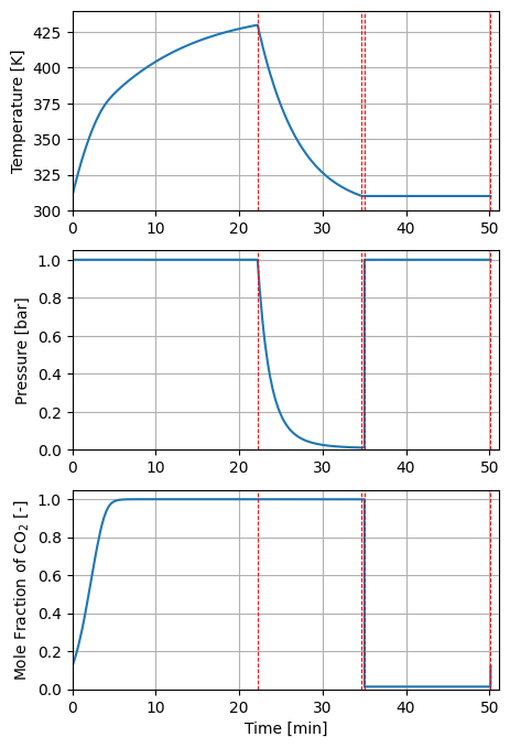
Step 5: Plotting Profiles#

Call plots method in the FixedBedTSA0D model to generate profiles of temperature, pressure and \(\mathrm{CO_{2}}\) concentration at the outlet of the column.

# profiles
plot_tsa_profiles(m.fs.tsa)

../../../_images/a8432d5129c58d38bd8f708febdd45153a375ed95cf1f529eef5f9e58a06cacc.png